Today, I finished the computing part and did exercises 4.1 and 4.2.
Computing:
#between-model comparisons
#set.seed(1056)
#logisticreg=train(Class~ ., data=GermanCreditTrain, method="glm",
# trcontrol=trainControl(method="repeatedcv", repeats=5))
#logisticreg
#resamp=resamples(list(SVM=svmfit, Logistic=logisticreg))
#summary(resamp)
#modeldifferences=diff(resamp)
#summary(modeldifference)
#kappa: sensitivity of output to changes or errors of input
Exercises 4.1 4.2
#choose data splitting method:
#nonrandom approaches
#random approaches: simple random sampling, stratified random sampling, maximum dissimilarity sampling
library(AppliedPredictiveModeling)
data(twoClassData)
str(predictors)
str(classes)
set.seed(1)
library(caret)
trainingrows=createDataPartition(classes, p=0.8, list=FALSE)
head(trainingrows)
trainpredictors=predictors[trainingrows, ]
trainclasses=classes[trainingrows]
testpredictors=predictors[-trainingrows, ]
testclasses=classes[-trainingrows]
trainpredictors
trainclasses
testpredictors
testclasses
Tomorrow, I will continue to do exercises of Chapter 4.
10/10/2016

10/07/2016
Computing2
Today, I practiced the Computing part of Chapter 4. They were about Basic Model Building in R and Determination of Tuning Parameters.
1.
#knn function in MASS
#ipredknn function in ipred
#knn3 function in caret
#formula interface: modelFunction(price ~ numBedrooms+numBaths+acres, data=housingData)
#non-formula interface: modelFunction(x=housePredictors, y=price)
library(caret)
trainpredictors=as.matrix(trainpredictors)
trainpredictors
knnfit=knn3(x=trainpredictors, y=trainclasses, k=5)
knnfit
#predict new samples
testpredictions=predict(knnfit, newdata = testpredictors, type = "class")
head(testpredictions)
2.
#e1071package contains the tune function
#errorest function in the ipred package
#the train function in the caret package
library(caret)
library(AppliedPredictiveModeling)
data("GermanCredit")
set.seed(100)
inTrain=createDataPartition(GermanCredit$Class, p = 0.8)[[1]]
GermanCreditTrain=GermanCredit[ inTrain, ]
GermanCreditTest=GermanCredit[-inTrain, ]
head(GermanCreditTrain)
head(GermanCreditTest)
set.seed(1056)
svmfit=train(Class~ .,data=GermanCreditTrain, method="svmRadial", preProc=c("center", "scale"),
tuneLength=10,
trControl=trainControl(method="repeatedcv", repeats=5, classProbs=TRUE))
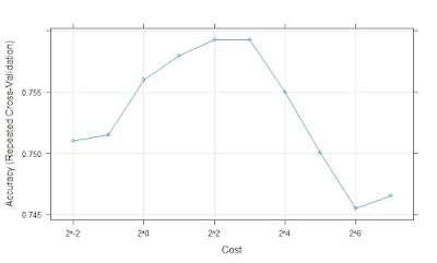
plot(svmfit, scales=list(x=list(log=2)))
predictedclasses=predict(svmfit, GermanCreditTest)
str(predictedclasses)
predictedprobs=predict(svmfit, newdata=GermanCreditTest, type="prob")
head(predictedprobs)
1.
#knn function in MASS
#ipredknn function in ipred
#knn3 function in caret
#formula interface: modelFunction(price ~ numBedrooms+numBaths+acres, data=housingData)
#non-formula interface: modelFunction(x=housePredictors, y=price)
library(caret)
trainpredictors=as.matrix(trainpredictors)
trainpredictors
knnfit=knn3(x=trainpredictors, y=trainclasses, k=5)
knnfit
#predict new samples
testpredictions=predict(knnfit, newdata = testpredictors, type = "class")
head(testpredictions)
2.
#e1071package contains the tune function
#errorest function in the ipred package
#the train function in the caret package
library(caret)
library(AppliedPredictiveModeling)
data("GermanCredit")
set.seed(100)
inTrain=createDataPartition(GermanCredit$Class, p = 0.8)[[1]]
GermanCreditTrain=GermanCredit[ inTrain, ]
GermanCreditTest=GermanCredit[-inTrain, ]
head(GermanCreditTrain)
head(GermanCreditTest)
set.seed(1056)
svmfit=train(Class~ .,data=GermanCreditTrain, method="svmRadial", preProc=c("center", "scale"),
tuneLength=10,
trControl=trainControl(method="repeatedcv", repeats=5, classProbs=TRUE))
plot(svmfit, scales=list(x=list(log=2)))
predictedclasses=predict(svmfit, GermanCreditTest)
str(predictedclasses)
predictedprobs=predict(svmfit, newdata=GermanCreditTest, type="prob")
head(predictedprobs)

Next week, I will continue to practice Computing.
10/06/2016
Chapter 4 (Computing)
Today, I did the Chapter 4 Computing. They were Data Splitting and Resampling.
library(AppliedPredictiveModeling)
data(twoClassData)
str(predictors)
str(classes)
set.seed(1)
library(caret)
trainingrows=createDataPartition(classes, p=0.8, list=FALSE)
head(trainingrows)
trainpredictors=predictors[trainingrows, ]
trainclasses=classes[trainingrows]
testpredictors=predictors[-trainingrows, ]
testclasses=classes[-trainingrows]
trainpredictors
trainclasses
testpredictors
testclasses
#maxdissim
#resampling
set.seed(1)
repeatedsplits=createDataPartition(trainclasses, p=0.8, time=3)
str(repeatedsplits)
#to create indicators for 10-fold cross-validation
set.seed(1)
cvsplits=createFolds(trainclasses, k=10, returnTrain = TRUE)
str(cvsplits)
fold1=cvsplits[[1]]
cvpredictors1=trainpredictors[fold1,]
cvclasses1=trainclasses[fold1]
nrow(trainpredictors)
nrow(cvpredictors1)
Tomorrow, I will do more on Computing.
library(AppliedPredictiveModeling)
data(twoClassData)
str(predictors)
str(classes)
set.seed(1)
library(caret)
trainingrows=createDataPartition(classes, p=0.8, list=FALSE)
head(trainingrows)
trainpredictors=predictors[trainingrows, ]
trainclasses=classes[trainingrows]
testpredictors=predictors[-trainingrows, ]
testclasses=classes[-trainingrows]
trainpredictors
trainclasses
testpredictors
testclasses
#maxdissim
#resampling
set.seed(1)
repeatedsplits=createDataPartition(trainclasses, p=0.8, time=3)
str(repeatedsplits)
#to create indicators for 10-fold cross-validation
set.seed(1)
cvsplits=createFolds(trainclasses, k=10, returnTrain = TRUE)
str(cvsplits)
fold1=cvsplits[[1]]
cvpredictors1=trainpredictors[fold1,]
cvclasses1=trainclasses[fold1]
nrow(trainpredictors)
nrow(cvpredictors1)
Tomorrow, I will do more on Computing.
10/05/2016
Chapter 4 (4.5-4.8)
Tuning parameters
It may be a good idea to favor simpler models over
more complex ones and choosing the tuning parameters based on the numerically
optimal value may lead to models that are overly complicated.
The fastest is 10-fold cross-validation. Repeated
cross-validation, the bootstrap, and repeated training-test splits fit the same
number of models and took about 5-fold more time to finish. LOOCV, which fits
as many models as there are samples in the training set, took 86-fold longer
and should only be considered when the number of samples is very small.
Data splitting
If the sample size is small: repeated 10-fold
cross-validation.
Reasons: The bias and variance properties are good
and, given the sample size, the computational cost are not large.
If the goal is to choose between models, a strong
case can be made for using one of the bootstrap procedures since they have very
low variance.
For large sample sizes, simple 10-fold
cross-validation should provide acceptable variance, low bias, and relatively
quick to compute.
Choosing between models
MARS: Multivariate adaptive regression splines
SVM: Support Vector Machine model
Sensitivity vs. Specificity
Tomorrow, I
will start computing in Chapter 4.
10/04/2016
Chapter 4 (4.3 4.4)
Today, I read the book “Applied Predictive Modeling”. I read the Chapter 4 (4.3 4.4).
Summary
Model building:
Pre-processing the predictor data
Estimating model parameters
Selecting predictors for the model
Evaluating model performance
Fine tuning class prediction rules
Resampling techniques often produce performance estimates superior to a single test set.
Nonrandom approaches
Random approaches
Simple random sampling
Stratified random sampling
Maximum dissimilarity sampling
Resampling techniques
k-fold cross-validation
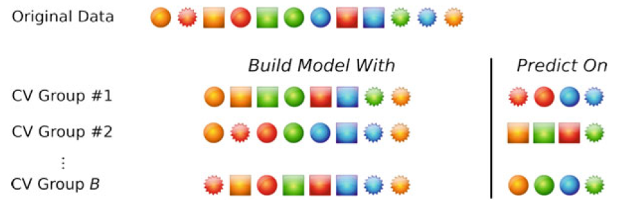
The samples are randomly partitioned into k sets of roughly equal size. A model is fit using the all samples except the first subset (called the first fold).
As k gets larger, the different in size between the training set and the resampling subsets gets smaller.
Repeating k-fold cross-validation can be used to effectively increase the precision of the estimates while still maintaining s small bias.

Generalized cross-validation
GCV=1/n ∑_(i=1)^n▒〖((y_i-y ̂_i)/(1-df/n))〗^2
df is the degrees of freedom of the model. The degrees of freedom are an accounting of how many parameters are estimated by the model(complexity for linear regression models).
Repeated Training/Test Splits
It is a function of the proportion of samples being randomly allocated to the prediction set; the larger the percentage, the more repetitions are needed to reduce the uncertainty in the performance estimates.

The Bootstrap
The bias will decrease as the training set sample size become larger.

Tomorrow, I will continue Chapter 4.
Summary
Model building:
Pre-processing the predictor data
Estimating model parameters
Selecting predictors for the model
Evaluating model performance
Fine tuning class prediction rules
Resampling techniques often produce performance estimates superior to a single test set.
Nonrandom approaches
Random approaches
Simple random sampling
Stratified random sampling
Maximum dissimilarity sampling
Resampling techniques
k-fold cross-validation
The samples are randomly partitioned into k sets of roughly equal size. A model is fit using the all samples except the first subset (called the first fold).
As k gets larger, the different in size between the training set and the resampling subsets gets smaller.
Repeating k-fold cross-validation can be used to effectively increase the precision of the estimates while still maintaining s small bias.

Generalized cross-validation
GCV=1/n ∑_(i=1)^n▒〖((y_i-y ̂_i)/(1-df/n))〗^2
df is the degrees of freedom of the model. The degrees of freedom are an accounting of how many parameters are estimated by the model(complexity for linear regression models).
Repeated Training/Test Splits
It is a function of the proportion of samples being randomly allocated to the prediction set; the larger the percentage, the more repetitions are needed to reduce the uncertainty in the performance estimates.
The Bootstrap
The bias will decrease as the training set sample size become larger.

Tomorrow, I will continue Chapter 4.
10/03/2016
Exercise 3 and Chapter 4 (4.1 4.2)
Today, I read the book “Applied Predictive
Modeling”. I practiced the exercise 3. I also read the Chapter 4 (4.1 4.2).
Exercise 3
library(caret)
data(BloodBrain)
logBBB
bbbDescr
library(e1071)
correlations=cor(bbbDescr)
library(corrplot)
corrplot(correlations)

Chpater 4 (4.1 4.2)
Over-fitting is a concern for any predictive model regardless of field of research.
In addition to learning the general patterns in the data, the model has also learned the characteristics of each sample’s unique noise. This type of model is said to be over-fit and will usually have poor accuracy when predicting a new sample.
A choice of too few neighbors may over-fit the individual points of the training set while too many neighbors may not be sensitive enough to yield reasonable performance. This type of model parameter is referred to as a tuning parameter because there is no analytical formula available to calculate an appropriate value.
‘cost’ parameter large: complicated model
‘cost’ parameter small: simple model
The apparent error rate can produce extremely optimistic performance estimates. A better approach is to test the model on samples that were not used for training.
Tomorrow, I will continue to read Chapter 4.
10/01/2016
Exercise 3.2
Today, I practised exercise 3.2. The following is the codes and results.
library(mlbench)
data(Soybean)
Soybean
library(caret)
head(Soybean)
Soybean$sever
sum(is.na(Soybean$sever))
na.omit(Soybean$sever)
sever = Soybean$sever
plot(sever,main="Sever Frequency Distribution", xlab="Sever", ylab="Frenquency")
sum(is.na(Soybean))
x=2337/683/35
x
summary(Soybean)
pmiss=function(sever){sum(is.na(sever))/length(sever)*100}
apply(Soybean, 2, pmiss)
library(mice)
library(VIM)
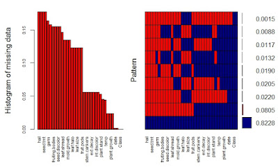
aggr_plot=aggr(Soybean, col=c('navyblue','red'), numbers=TRUE, sortVars=TRUE, labels=names(Soybean), cex.axis=0.7, gap=2.5, ylab=c("Histogram of missing data","Pattern"))
tempSoybean=mice(Soybean,m=35,maxit=50,meth='pmm',seed=500)

Next week, I will continue to practise exercises in the book.
library(mlbench)
data(Soybean)
Soybean
library(caret)
head(Soybean)
Soybean$sever
sum(is.na(Soybean$sever))
na.omit(Soybean$sever)
sever = Soybean$sever
plot(sever,main="Sever Frequency Distribution", xlab="Sever", ylab="Frenquency")
sum(is.na(Soybean))
x=2337/683/35
x
summary(Soybean)
pmiss=function(sever){sum(is.na(sever))/length(sever)*100}
apply(Soybean, 2, pmiss)
library(mice)
library(VIM)
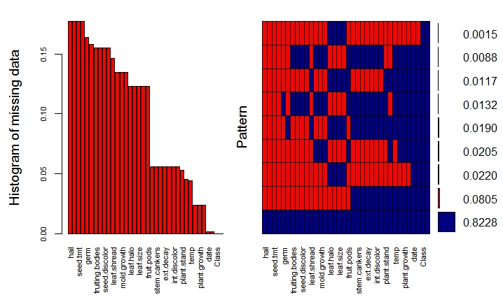
aggr_plot=aggr(Soybean, col=c('navyblue','red'), numbers=TRUE, sortVars=TRUE, labels=names(Soybean), cex.axis=0.7, gap=2.5, ylab=c("Histogram of missing data","Pattern"))
tempSoybean=mice(Soybean,m=35,maxit=50,meth='pmm',seed=500)

Next week, I will continue to practise exercises in the book.
Subscribe to:
Posts (Atom)