Chapter 7 application (7.2)

Today, I read Chapter 7 (7.2) and find something useful for my research.

Summary

MARS: Multivariate Adaptive Regression Splines

GCV: generalized cross-validation

There are two tuning parameters associated with the MARS model: the degree of the features that are added to the model and the number of retained terms. The latter parameter can be automatically determined using the default pruning procedure (using GCV), set by the user or determined using an external resampling technique.

There are several advantages to using MARS. First, the model automatically conducts feature selection; the model equation is independent of predictor variables that are not involved with any of the final model features. This point cannot be underrated. Given a large number of predictors seen in many problem domains, MARS potentially thins the predictor set using the same algorithm that builds the model. In this way, the feature selection routine has a direct connection to functional performance. The second advantage is interpretability. Each hinge feature is responsible for modeling a specific region in the predictor space using a (piecewise) linear model. When the MARS model is additive, the contribution of each predictor can be isolated without the need to consider the others. This can be used to provide clear interpretations of how each predictor relates to the outcome. For nonadditive models, the interpretive power of the model is not reduced. Finally, the MARS model requires very little pre-processing of the data; data transformations and the filtering of predictors are not needed.

Another method to help understand the nature of how the predictors affect the model is to quantify their importance to the model. For MARS, one technique for doing this is to track the reduction in the root mean squared error (as measured using the GCV statistic) that occurs when adding a particular feature to the model.

The following figure compares the predictors and we can see the importance of predictors from the figure.

Tomorrow, I will continue to read the book.

Chapter 7 application (7.1)

Today, I read Chapter 7 (7.1) to find something useful for my research.

Summary

Nonlinear Regression Models

Neural Networks

Weight decay is an approach to moderate over-fitting. It is a penalization method to regularize the model similar to ridge regression.

As the regularization value λ increases, the fitted model becomes more smooth and less likely to over-fit the training set.

Of course, the value of this parameter must be specified and, along with the number of hidden units, is a tuning parameter for the model. Reasonable values of λ range between 0 and 0.1. Also note that since the regression coefficients are being summed, they should be on the same scale; hence the predictors should
be centered and scaled prior to modeling.

Neural networks are models which are more accurate than linear models. It can be used to be applied to the log data. After building the data matrix, we may have dozens of predictors, namely log data to predict outcomes, namely NMR data. Before building the model , we can first center and scale predictors and use PCA to decrease correlations between every pair of predictors. Then we can set a set of tuning parameters of weight decay and number of hidden units to build the model. After running the codes, we can find the optimized tuning parameter so that  we can choose the optimized neural network model. It may perform well in predicting NMR data.

If we can just find the local optimization but not the global one, we can use the model averaged neural networks to solve the problem. The approach is that we start do modeling with several different starting numbers so that we can get different results of the model. Then we average them to get the more reliable results.

The following is an example of the comparison of neural networks with different tuning parameters.

Tomorrow, I will continue to read the book.

Chapter 6 Application (6.4&6.5)

Today, I finished reading Chapter 6 to find something useful for my research.

Summary

Because the dimension reduction offered by PLS is supervised by the response, it is more quickly steered towards the underlying relationship between the predictors and the response.

NIPALS: nonlinear iterative partial least squares algorithm

The constructs of NIPALS could be obtained by working with a “kernel” matrix of dimension P × P, the covariance matrix of the predictors (also of dimension P×P), and the covariance matrix of the predictors and response (of dimension P ×1). This adjustment improved the speed of the algorithm, especially as the number of observations became much larger than the number of predictors.

SIMPLS: simple modification of the PLS algorithm.

If a more intricate relationship between predictors and response exists, then we suggest employing one
of the other techniques rather than trying to improve the performance of PLS through this type of augmentation.

Partial least square regression vs. Ordinary least square regression

Penalized models

Combatting collinearity by using biased models may result in regression models where the overall MSE
is competitive.

One method of creating biased regression models is to add a penalty to the sum of the squared errors.

Ridge regression adds a penalty on the sum of the squared regression parameters:

Penalty increase, bias increase, variance decrease, model under-fit.

Lasso: least absolute shrinkage and selection operator model

A generalization of the lasso model is the elastic net. This model combines the two types of penalties:

The advantage of this model is that it enables effective regularization via the ridge-type penalty with the feature selection quality of the lasso penalty.

Tomorrow, I will continue to read Chapter 7 of the book.

Review of Codes

Today, I review the codes of the book from Chapter 3 to Chapter 5.

I think that I forget some of the codes when I read the book, so I decide to spend some time reviewing them.

Summary

#Coefficient of determination (R^2): the proportion of the information in the data that is explained by the model.
#It is a measure of correlation, not accuracy. It is dependent on the variation in the outcome. Same RMSE, larger variance, larger R^2.
observed=c(0.22, 0.83, -0.12, 0.89, -0.23, -1.30, -0.15, -1.4, 0.62, 0.99, -0.18, 0.32, 0.34,
           -0.3, 0.04, -0.87, 0.55, -1.3, -1.15, 0.2)
predicted=c(0.24, 0.78, -0.66, 0.53, 0.7, -0.75, -0.41, -0.43, 0.49, 0.79, -1.19, 0.06, 0.75,
           -0.07, 0.43, -0.42, -0.25, -0.64, -1.26, -0.07)
#in practice, the vector of predictions would be produced by the model function
residualvalues=observed-predicted
residualvalues
summary(residualvalues)
axisrange=extendrange(c(observed, predicted))
plot(observed, predicted, ylim=axisrange, xlim=axisrange)
abline(0, 1, col="darkgrey", lty=2)
plot(predicted, residualvalues, ylab = "residual")
abline(h=0, col="darkgrey", lty=2)
library(caret)
R2(predicted, observed)
RMSE(predicted, observed)
cor(predicted, observed)
cor(predicted, observed, method = "spearman")

library(AppliedPredictiveModeling)
data(twoClassData)
str(predictors)
str(classes)
set.seed(1)
library(caret)
trainingrows=createDataPartition(classes, p=0.8, list=FALSE)
head(trainingrows)
trainpredictors=predictors[trainingrows, ]
trainclasses=classes[trainingrows]
testpredictors=predictors[-trainingrows, ]
testclasses=classes[-trainingrows]
trainpredictors
trainclasses
testpredictors
testclasses
#maxdissim
#resampling
set.seed(1)
repeatedsplits=createDataPartition(trainclasses, p=0.8, time=3)
str(repeatedsplits)
#to create indicators for 10-fold cross-validation
set.seed(1)
cvsplits=createFolds(trainclasses, k=10, returnTrain = TRUE)
str(cvsplits)
fold1=cvsplits[[1]]
cvpredictors1=trainpredictors[fold1,]
cvclasses1=trainclasses[fold1]
nrow(trainpredictors)

nrow(cvpredictors1)

#e1071package contains the tune function
#errorest function in the ipred package
#the train function in the caret package
library(caret)
library(AppliedPredictiveModeling)
data("GermanCredit")
set.seed(100)
inTrain=createDataPartition(GermanCredit$Class, p = 0.8)[[1]]
inTrain
GermanCreditTrain=GermanCredit[ inTrain, ]
GermanCreditTest=GermanCredit[-inTrain, ]
head(GermanCreditTrain)
head(GermanCreditTest)
set.seed(1056)
svmfit=train(Class~ .,data=GermanCreditTrain, method="svmRadial", preProc=c("center", "scale"), 
             tuneLength=10, 
             trControl=trainControl(method="repeatedcv", repeats=5, classProbs=TRUE))
svmfit
#first method: classification or regression model
#train control: the resampling method
#tuneLength: an integer denoting the amount of granularity in the tuning parameter grid
plot(svmfit, scales=list(x=list(log=2)))
predictedclasses=predict(svmfit, GermanCreditTest)
str(predictedclasses)
predictedprobs=predict(svmfit, newdata=GermanCreditTest, type="prob")
head(predictedprobs)
#between-model comparisons
#set.seed(1056)
#logisticreg=train(Class~ ., data=GermanCreditTrain, method="glm",
#            trcontrol=trainControl(method="repeatedcv", repeats=5))
#logisticreg
#resamp=resamples(list(SVM=svmfit, Logistic=logisticreg))
#summary(resamp)
#modeldifferences=diff(resamp)
#summary(modeldifference)

#kappa: sensitivity of output to changes or errors of input

Next week, I will continue to read the book.

Chapter 6.3 application

Today, I read Chapter 6 (6.3) and find something which could be useful for my research.

Summary

Partial Least Squares

The removal of highly correlated pairwise predictors may not guarantee a stable least squares solution. Alternatively, using PCA for pre-processing guarantees that the resulting predictors, or combinations thereof, will be uncorrelated.

Pre-processing predictors via PCA prior to performing regression in known as principal component regression (PCR).

If the variability in the predictor space is not related to the variability of the response, then PCR can have difficulty identifying a predictive relationship when one might actually exist. Because of this, it is recommended to use PLS when there are correlated predictors and a linear regression-type solution is desired.

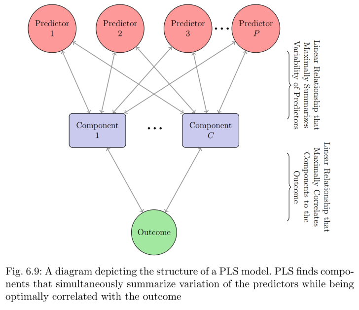
While the PCA linear combinations are chosen to maximally summarize predictor space variability, the PLS linear combinations of predictors are chosen to maximally summarize covariance with the response. This means that PLS finds components that maximally summarize the variation of the predictors while simultaneously requiring these components to have maximum correlation with the response. (predictors-components-response)

PLS has one tuning parameter: the number of components to retain.

Tomorrow, I will continue to read the book.

Chapter 5&6(6.1 6.2) application

Today, I read Chapter 5&6(6.1 6.2) to find something useful which could be used in my research.

Summary

Chapter 5 Application

Quantitative measures of performance

RMSE: the square root of MSE so that it is in the same units as the original data

: the proportion of the information in the data that is explained by the model. It is a measure of correlation, not accuracy.

The variance-bias trade-off: high variance or high bias, that is a question. Increasing bias can reduce model variance.

Chapter 6 Application

Ordinary linear regression finds parameter estimates that have minimum bias, whereas ridge regression, the lasso, and the elastic net find estimates that have lower variance.

Linear regression:

SSE: sum-of-squared errors.

When there are highly correlated predictors, we should remove one of the offending predictors or find models which can tolerate collinearity.

Tomorrow, I will read more of the book to frame questions.

Chapter 4 application

Today, I read Chapter 4 to find something which could be used in my research.

Summary

Over-fitting

Model tuning: tune an appropriate value of a tuning parameter

Data splitting: maximum dissimilarity sampling

Common steps in model building:

1.      Pre-processing the predictor data

2.      Estimating model parameters

3.      Selecting predictors for the model

4.      Evaluating model performance

5.      Fine tuning class prediction rules (via ROC curves, etc)

Resampling techniques:

1.      K-fold cross validation

2.      Generalized cross validation (approximate the leave-one-out error rate)

For example, in the last leave-one-out cross validation, df=1 and n=12.

3.      Repeated training/testing splits

4.      Bootstrap

Choose final tuning parameters with different considerations of various factors

Choosing between models:
1. Start with several models that are the least interpretable and most flexible.

2. investigate simpler models that are less opaque

3. consider using simplest model that reasonably approximates the performance of the more complex methods