11/28/2016

Chapter 3 application 2

Today, I finished reading chapter 3 and found something which could be applied to my research. In addition, I looked into IP to try to know what do all the data mean. I have known some of them basically.

Summary


Tomorrow, I will read chapter 4 to find more information which may be useful for my research.

11/22/2016

Chapter 3 application

Today, I browsed the rest of the paper and started to look into the data. There are many ways of data pre-processing in chapter 3 and they can be applied into the log data.

Summary

paper:


Chapter 3:
1. Individual predictors:
Centering: the predictor has a zero mean
Scaling: each value of the predictor variable is divided by its standard deviation. Scaling the data coerce the values to have a common standard deviation of one.
Removing skewness: Box-Cox transformation

After holiday, I will start to frame questions of each chapter and try to apply them into the data.


11/21/2016

Preparing for using data

Today, I started to look into data in IP and tried to be familiar with IP software. Also, Yifu gave me a paper which is written by the people from Hess Corporation. I read a little of it.

Summary
SPWLA paper
TOC: total organic carbon

According the paper, the lithology is very complicated. I think if I need to predict NMR permeability with R method, the lithology of the data and the lithology of where I need to predict should be similar.


Tomorrow, I will continue to read the paper and look into the data.

11/18/2016

Chapter 10 (Computing finished)

Today, I fixed some problems of computing of Chapter 10.

Codes:
pp2=preProcess(age28data[, 1:7], "pca")
pca1=predict(pp2, age28data[, 1:7])
head(pca1)
pca1$Data="Training Set"
pca1$Data[startpoints]="Starting Values"
pca3=predict(pp2, cbresults[, 1:7])
pca3$Data="Cubist"
head(pca3)
pca4=predict(pp2, nnetresults[, 1:7])
pca4$Data="Neural Network"
head(pca4)
pcadata=rbind(pca1, pca3, pca4)
dim(pcadata)
pcadata$Data=factor(pcadata$Data,
                    levels = c("Training Set","Starting Values",
                    "Cubist","Neural Network"))
lim=extendrange(pcadata[, 1:2])

# convert a vector of strings into a vector of numbers
m=with(pcadata, as.numeric(levels(factor(as.numeric(factor(pcadata$Data))))))
m=with(pcadata, levels(factor(Data)))
m
colm=c()
for(i in 1:length(pcadata$Data))
{
  colm[i]=which(pcadata$Data[i]==m)
}
colm

xyplot(PC2 ~ PC1, data = pcadata, groups = Data,
       auto.key = list(columns = 2),
       xlim = lim, ylim = lim,
       col=colm,
       type = c("g", "p")
      )

xyplot(PC2 ~ PC1, data = pcadata, groups = Data,
       auto.key = list(columns = 2),
       xlim = lim, ylim = lim,
       col=c("blue", "pink", "red", "green"),
       type = c("g", "p")
)

Next week, I will start to look into the NMR data.

11/17/2016

Chapter 10 computing

Today, I did computing of Chapter 10.

Codes:
modelPrediction=function(x, mod)
{
  if(x[1] < 0 | x[1] > 1) return(10^38)
  if(x[2] < 0 | x[2] > 1) return(10^38)
  if(x[3] < 0 | x[3] > 1) return(10^38)
  if(x[4] < 0 | x[4] > 1) return(10^38)
  if(x[5] < 0 | x[5] > 1) return(10^38)
  if(x[6] < 0 | x[6] > 1) return(10^38)
  x=c(x, 1 - sum(x))
  if(x[7] < 0.05) return(10^38)
  tmp <- as.data.frame(t(x))
  names(tmp)=c('Cement','BlastFurnaceSlag','FlyAsh',
               'Superplasticizer','CoarseAggregate',
               'FineAggregate', 'Water')
  tmp$Age=28
  -predict(mod, tmp)
}

# Cubist mdoel
cbresults=startingvalues
cbresults$Water=NA
cbresults$Prediction=NA
cbresults
for(i in 1:nrow(cbresults))
{
  results=optim(unlist(cbresults[i,1:6]),
                     modelPrediction,
                     method = "Nelder-Mead",
                    control=list(maxit=5000),
                      mod = cbmodel)
  cbresults$Prediction[i]=-results$value
  # save the final mixture values
  cbresults[i,1:6]=results$par
}
#col.sums <- apply(x, 2, sum)  row.sums <- apply(x, 1, sum)  rbind  cbind
cbresults$Water=1 - apply(cbresults[,1:6], 1, sum)
# Keep the top three mixtures, -: decreasing order
cbresults=cbresults[order(-cbresults$Prediction),][1:3,]
cbresults$Model="Cubist"
cbresults

       Cement BlastFurnaceSlag      FlyAsh Superplasticizer CoarseAggregate FineAggregate      Water Prediction  Model
523 0.1747206       0.17969922 0.012880890     0.0027363548       0.3200175     0.2532112 0.05673427  102.44370 Cubist
495 0.2098331       0.05295034 0.006751067     0.0003692619       0.3538669     0.3238973 0.05233208   86.01767 Cubist
477 0.2110388       0.04514574 0.062017524     0.0023323792       0.3178446     0.3077021 0.05391885   85.51025 Cubist

# neural network model
nnetresults=startingvalues
nnetresults$Water=NA
nnetresults$Prediction=NA
nnetresults
for(i in 1:nrow(nnetresults))
{
  results=optim(unlist(nnetresults[i,1:6]),
                modelPrediction,
                method = "Nelder-Mead",
                control=list(maxit=5000),
                mod = nnetmodel)
  nnetresults$Prediction[i]=-results$value
  nnetresults[i,1:6]=results$par
}
nnetresults$Water=1 - apply(nnetresults[,1:6], 1, sum)
nnetresults=nnetresults[order(-nnetresults$Prediction),][1:3,]
nnetresults$Model="NNet"
nnetresults

       Cement BlastFurnaceSlag       FlyAsh Superplasticizer CoarseAggregate FineAggregate      Water Prediction Model
69  0.1617514       0.13291706 5.509921e-10      0.007644831       0.3905959     0.2564540 0.05063673   81.92797  NNet
357 0.1366392       0.04989215 2.395829e-08      0.002012726       0.4513948     0.3012054 0.05885566   80.16362  NNet
477 0.2145572       0.04306283 4.614330e-02      0.001330241       0.2993219     0.3299018 0.06568276   79.59500  NNet
(I am faced with some problems of drawing graphs. Tomorrow, I will try to fix them.)

Tomorrow, I will fix some problems of the codes.

11/16/2016

Chapter 10 computing

Today, I continued to do computing of Chapter 10.

Codes:
# plot the RMSE values
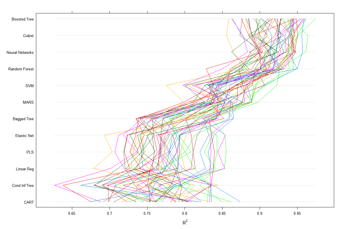
parallelplot(allresamples)
# using R2
parallelplot(allresamples, metric="Rsquared")


nnetpredictions=predict(nnetmodel, testset)
gbmpredictions=predict(gbmmodel, testset)
cbpredictions=predict(cbmodel, testset)

age28data=subset(trainingset, Age==28)
dim(age28data)
# remove the age and compressive strength columns and
# then center and scale the predictor columns
pp1=preProcess(age28data[,-(8:9)], c("center", "scale"))
scaledtrain=predict(pp1, age28data[, 1:7])
dim(scaledtrain)
# a single random mixture is selected to initialize the maximum dissimilarity sampling process
set.seed(91)
startmixture=sample(1:nrow(age28data), 1)
starters=scaledtrain[startmixture, 1:7]
#select 14 more mixtures to complete a diverse set of starting points for the search algorithms
library(proxy)
maxdis=maxDissim(starters, scaledtrain, 14)
maxdis
startpoints=c(startmixture, maxdis)
starters=age28data[startpoints, 1:7]
starters
# all seven mixture proportions should add to one
# the water proportion will be determined by the sum of the other six ingredient proportions
# remove water
startingvalues=starters[, -4]

Tomorrow, I will continue to do computing of Chapter 10.

11/15/2016

Chapter 10 computing

Today, I did computing of Chapter 10.

Codes:
library(AppliedPredictiveModeling)
data(concrete)
str(concrete)
str(mixtures)
library(Hmisc)
library(caret)
# g: grid; p: points; smooth: smoother between: add space between panels.
featurePlot(x=concrete[,-9], y=concrete$CompressiveStrength,
            between=list(x=1, y=1),
            type=c("g", "p", "smooth"))
# ? averaging the replicated mixtures and splitting the data into training and test sets
library(plyr)
averaged=ddply(mixtures, .(Cement, BlastFurnaceSlag, FlyAsh, Water, Superplasticizer, CoarseAggregate,
                           FineAggregate, Age), function(x) c(CompressiveStrength=mean(x$CompressiveStrength)))
str(averaged)
set.seed(975)
fortraining=createDataPartition(averaged$CompressiveStrength, p=3/4)[[1]]
trainingset=averaged[fortraining,]
testset=averaged[-fortraining,]
dim(trainingset)
dim(testset)
# The dot in the formula below is shorthand for all predictors and
# (.)^2 expands into a model with all the linear terms and all two-factor interactions.
modformula=paste("CompressiveStrength ~ (.)^2 + I(Cement^2) + ",
                 "I(BlastFurnaceSlag^2)+I(FlyAsh^2)+I(Water^2)+",
                 "I(Superplasticizer^2)+I(CoarseAggregate^2)+",
                 "I(FineAggregate^2)+I(Age^2)")
modformula=as.formula(modformula)
modformula
# the predictors' number of modformula is different from the book, but after the test of a different one, modformula2,
modformula2=paste("CompressiveStrength ~ (.)^2")
modformula2=as.formula(modformula2)
modformula2
# modformula and modformula2 have different results of linearreg although their predictors' numbers are the same.
# so I guess that modformula is correct.
controlobject=trainControl(method="repeatedcv", repeats=5, number=10)
set.seed(669)
linearreg=train(modformula, data=trainingset, method="lm", trControl=controlobject)
linearreg

# the other two linear models were created
set.seed(669)
plsmodel=train(modformula, data=trainingset, method="pls", preProcess = c("center", "scale"),
               tuneLength = 15, trControl = controlobject)
plsmodel
# centered (44) and scaled (44): 44 is right.
library(elasticnet)
enetgrid2=expand.grid(.lambda=c(0, 0.001, 0.01, 0.1),
                      .fraction=seq(0.05, 1, length=20))
set.seed(669)
enetmodel2=train(modformula, data=trainingset, method="enet", preProcess = c("center", "scale"),
                 tuneGrid=enetgrid2, trControl=controlobject)
enetmodel2

# MARS
library(earth)
set.seed(669)
earthmodel=train(CompressiveStrength~., data=trainingset, method="earth",
                 tuneGrid=expand.grid(.degree=1, .nprune=2:25), trControl=controlobject)
earthmodel

#SVMs
library(kernlab)
set.seed(669)
svmmodel=train(CompressiveStrength~., data=trainingset, method="svmRadial",
               tuneLength=15, preProcess=c("center", "scale"), trControl=controlobject)
svmmodel

# Neural Networks
library(nnet)
nnetgrid=expand.grid(.decay=c(0.001, 0.01, 0.1), .size=seq(1, 27, by=2), .bag=FALSE)
set.seed(669)
nnetmodel=train(CompressiveStrength~., data=trainingset, method="avNNet",
                tuneGrid=nnetgrid, preProcess=c("center", "scale"),
                linout=TRUE, trace=FALSE, maxit=1000, trControl=controlobject)
nnetmodel

# regression and model trees
library(rpart)
set.seed(669)
rpartmodel=train(CompressiveStrength~., data=trainingset, method="rpart",
                 tuneLength=30, trControl=controlobject)
rpartmodel

set.seed(669)
library(party)
ctreemodel=train(CompressiveStrength~., data=trainingset, method="ctree",
                 tuneLength=10, trControl=controlobject)
ctreemodel

set.seed(669)
library(RWeka)
mtmodel=train(CompressiveStrength~., data=trainingset, method="M5",
              trControl=controlobject)
mtmodel

# remaining model objects
library(ipred)
library(plyr)
library(e1071)
set.seed(669)
treebagmodel=train(CompressiveStrength~., data=trainingset, method="treebag",
                   trControl=controlobject)
treebagmodel

library(randomForest)
set.seed(669)
rfmodel=train(CompressiveStrength~., data=trainingset, method="rf",
              tuneLength=7, ntrees=1000, importance=TRUE,
              trControl=controlobject)
rfmodel

gbmgrid=expand.grid(.interaction.depth = seq(1, 7, by = 2),
                    .n.trees = seq(100, 1000, by = 50),
                    .shrinkage = c(0.01, 0.1), .n.minobsinnode=10)
library(gbm)
set.seed(669)
gbmmodel=train(CompressiveStrength~., data=trainingset, method="gbm",
               tuneGrid=gbmgrid, verbose=FALSE, trControl=controlobject)
gbmmodel

cubistgrid=expand.grid(.committees = c(1, 5, 10, 50, 75, 100),
                       .neighbors = c(0, 1, 3, 5, 7, 9))
library(Cubist)
set.seed(669)
cbmodel=train(CompressiveStrength~., data=trainingset, method="cubist",
              tuneGrid=cubistgrid, trControl=controlobject)
cbmodel
allresamples=resamples(list("Linear Reg"=lmmodel), "PLS"=plsmodel,
                       "Elastic Net"=enetmodel2, "MARS"=earthmodel,
                       "SVM"=svmmodel,
                       # "Neural Networks"=nnetmodel,
                       "CART"=rpartmodel, "Cond Inf Tree" = ctreemodel,
                       "Bagged Tree" = treebagmodel, "Boosted Tree" = gbmmodel,
                       "Random Forest" = rfmodel, "Cubist" = cbmodel))
(There should be a figure of comparison among these models. However, the nnetmodel takes so much time to calculate that it has not shown the result till now. I will keep it calculating all the night and it should show the result tomorrow.)

Tomorrow, I will continue to do computing of Chapter 10.