Chapter 10 (10.1 10.2 10.3)

Today, I read Chapter 10 (10.1 10.2 10.3) and started to do computing of Chapter 10.

Summary

Case Study: Compressive Strength of Concrete Mixtures

A balanced design is one where no one experimental factor (i.e., the predictors) has more focus than the others. In most cases, this means that each predictor has the same number of possible levels and that the frequencies of the levels are equivalent for each factor.

Sequential experimentation

1.     Screen a large number of possible experimental factors to determine important factors

2.     More focused experiments are created with subset of important factors

3.     The nature of relationship between the important factors can be further elucidated

4.     Fine-tune a small number of important factors

In this chapter, models will be created to help find potential recipes to maximize compressive strength.

Model Building Strategy

A data splitting approach will be taken for this case study. A random holdout set of 25 % (n = 247) will be used as a test set and five repeats of 10-fold cross-validation will be used to tune the various models。

Model Performance

The top performing models were tree ensembles (random forest and boosting), rule ensembles (Cubist), and neural networks.

Optimizing Compressive Strength

Many rely on determining the gradient (i.e., first derivative) of the prediction equation. Several of the models have smooth prediction equations (e.g., neural networks and SVMs).

Neural networks: smooth model

Cubist: non-smooth model

Computing

library(AppliedPredictiveModeling)

data(concrete)

str(concrete)

str(mixtures)

library(Hmisc)

library(caret)

# g: grid; p: points; smooth: smoother between: add space between panels.

featurePlot(x=concrete[,-9], y=concrete$CompressiveStrength,

            between=list(x=1, y=1),

            type=c("g", "p", "smooth"))

#averaging the replicated mixtures and splitting the data into training and test sets

library(plyr)

averaged=ddply(mixtures, .(Cement, BlastFurnaceSlag, FlyAsh, Water, Superplasticizer, CoarseAggregate,

                           FineAggregate, Age), function(x) c(CompressiveStrength=mean(x$CompressiveStrength)))

str(averaged)

set.seed(975)

fortraining=createDataPartition(averaged$CompressiveStrength, p=3/4)[[1]]

trainingset=averaged[fortraining,]

testset=averaged[-fortraining,]

Tomorrow, I will continue to do computing of Chapter 10.

Chapter 9

Today, I read Chapter 9.

Summary

A Summary of Solubility Models

With the exception of poorly performing models, there is a fairly high correlation between the results derived from resampling and the test set (0.9 for the RMSE and 0.88 for R2).

There was a “pack” of models that showed better results, including model trees, linear regression, penalized linear models, MARS, and neural networks.

The group of high-performance models include support vector machines (SVMs), boosted trees, random forests, and Cubist.

There are very few statistically significant differences among high-performance models. Given this, any of these models would be a reasonable choice.

Next week, I will read Chapter 10, which is the last chapter of Part 2 of the book. After finishing Chapter 10, I think it is time to apply them into the real data.

Chapter 8 Exercises

Today, I finished exercises of Chapter 8.

# 8.5
library(caret)
data(tecator)
absorp
# moisture fat protein
endpoints
absorpchange=absorp
dim(absorpchange)
absorpchange2=cbind(absorpchange, moisture=endpoints[,1])
absorpchange2=data.frame(absorpchange2)
library(RWeka)
treemodel1=M5P(moisture~., data=absorpchange2)
plot(treemodel1)

set.seed(100)
treemodel2=train(absorpchange2[,1:100], absorpchange2$moisture, method="M5", trControl = trainControl(method = "cv"),
             control= Weka_control(M=10))
treemodel2 # RMSE min = 6.5
plot(treemodel2)
toohigh=findCorrelation(cor(absorpchange2[,1:100]), cutoff = 0.999)
toohigh
trainabsorp=absorpchange2[,-toohigh]
treemodel3=M5P(moisture~., data=trainabsorp)
plot(treemodel3)

set.seed(100)
treemodel4=train(trainabsorp[,1:4], trainabsorp$moisture, method="M5", trControl = trainControl(method = "cv"),
                 control= Weka_control(M=10))
treemodel4 # RMSE min = 6.0
plot(treemodel4)

 

# 8.6
library(AppliedPredictiveModeling)
data(permeability)
dim(fingerprints)
permeability
library(caret)
lowfrequencies=nearZeroVar(fingerprints, freqCut = 20, uniqueCut = 10)
fingerfiltered=fingerprints[, -lowfrequencies]
dim(fingerfiltered)
library(randomForest)
rfmodel=randomForest(permeability~., data=fingerfiltered)
plot(rfmodel)
rfmodel2=randomForest(fingerfiltered, permeability, importance = TRUE, ntrees=1000)
plot(rfmodel2)
imp=importance(rfmodel2)
# %IncMSE: the higher number, the more important
# IncNodePurity: More useful variables achieve higher increases in node purities

Tomorrow, I will read Chapter 9.

Chapter 8 (Computing & Exercises)

Today, I finished Computing and did exercises of Chapter 8.

Computing
# 5. Boosted Trees (gbm: gradient boosting machines)
library(gbm)
gbmmodel=gbm.fit(solTrainXtrans, solTrainY, distribution = "gaussian")
gbmmodel=gbm(y~., data=trainData, distribution = "gaussian")
# The furthest you can go is to split each node until there is only 1 observation in each terminal node.
# This would correspond to n.minobsinnode=1.
gbmgrid=expand.grid(.interaction.depth=seq(1, 7, by=2), .n.minobsinnode=10,
                    .n.trees=seq(100, 1000, by=50), .shrinkage=c(0.01, 0.1))
set.seed(100)
gbmtune=train(solTrainXtrans, solTrainY, method="gbm", tuneGrid = gbmgrid, verbose=FALSE)
gbmtune
system.time(gbmtune)

# 6. Cubist
library(Cubist)
# an argument, committees, fits multiple models
cubistmodel=cubist(solTrainXtrans, solTrainY, committees = 5)
cubistmodel
# an argument, neighbors,can take on a single integer value (0-9) to
# adjust the rule-based predictions from the training set
cubistpred=predict(cubistmodel, solTestXtrans)
summary(cubistpred)
head(cubistpred)
# the train function in the caret package can tune the model over values of
# committees and neighbors through resampling
cubisttuned=train(solTrainXtrans, solTrainY, method="cubist")
cubisttuned

Exercises
library(mlbench)
set.seed(200)
simulated=mlbench.friedman1(200, sd=1)
simulated=cbind(simulated$x, simulated$y)
simulated=as.data.frame(simulated)
colnames(simulated)[ncol(simulated)]="y"
head(simulated)
library(randomForest)
library(caret)
model1=randomForest(y~., data=simulated, importance=TRUE, ntree=1000)
rfimp1=varImp(model1, scale=FALSE)
rfimp1
simulated$duplicate1=simulated$V1+rnorm(200)*0.1
cor(simulated$duplicate1, simulated$V1)
model2=randomForest(y~., data=simulated, importance=TRUE, ntree=1000)
rfimp2=varImp(model2, scale=FALSE)
rfimp2
library(party)
model3ctr=cforest_control(mtry=ncol(simulated)-1)
model3tree=cforest(y~., data=simulated, controls = model3ctr)
model3tree
cfimp=varimp(model3tree)
cfimp

Tomorrow, I will continue to do exercises of Chapter 8.

Chapter 8 Computing

Today, I did Computing of Chapter 8.

Summary
# the R packages used in this section are caret, Cubist, gbm, ipred, party, partykit,
# randomForest, rpart, RWeka

# 1. Single Trees

# formula method
library(rpart)
rparttree=rpart(y~., data=trainData)
library(party)
ctreetree=ctree(y~., data=trainData)

library(caret)
set.seed(100)
rparttune1=train(solTrainXtrans, solTrainY, method="rpart2", tuneLength=12, trControl=trainControl(method="cv"))
rparttune1
set.seed(100)
rparttune2=train(solTrainXtrans, solTrainY, method="rpart", tuneLength=10, trControl=trainControl(method="cv"))
rparttune2
?rpart.control
?ctree_control
plot(rparttune1)
plot(rparttune2)

library(partykit)
# convert the rpart object to a party object
rparttree2=as.party(rparttree)
plot(rparttree2)

# 2. Model Trees
library(RWeka)

# formula method
m5tree=M5P(y~., data=trainData)
m5rules=M5Rules(y~., data=trainData)

set.seed(100)
m5tune=train(solTrainXtrans, solTrainY, method="M5", trControl = trainControl(method = "cv"),
# M=10 is the minimum number of samples needed to further splits the data to be 10
             control= Weka_control(M=10))
plot(m5tune)

# 3. Bagged Trees
library(ipred)
# bagging uses the formula interface and ipredbagg has the non-formula interface
baggedtree=ipredbagg(solTrainY, solTrainXtrans)
baggedtree=bagging(y~., data = trainData)
baggedtree2=as.party(baggedtree)

# mtry is equal to the number of predictors
bagctr1=cforest_control(mtry=ncol(trainData)-1)
baggedtree=cforest(y~., data=trainData, controls = bagCtr1)

# 4. Random Forest
library(randomForest)
rfmodel=randomForest(solTrainXtrans, solTrainY)
rfmodel=randomForest(y~., data=trainData)
plot(rfmodel)
# the default for mtry in regression is the number of prediction divided by 3
rfmodel2=randomForest(solTrainXtrans, solTrainY, importance = TRUE, ntrees=1000)
plot(rfmodel2)
importance(rfmodel2)

Tomorrow, I will continue to do computing of Chapter 8.

Chapter 8 (8.5 8.6 8.7)

Today, I read Chapter 8 (8.5 8.6 8.7) of the book.

Summary
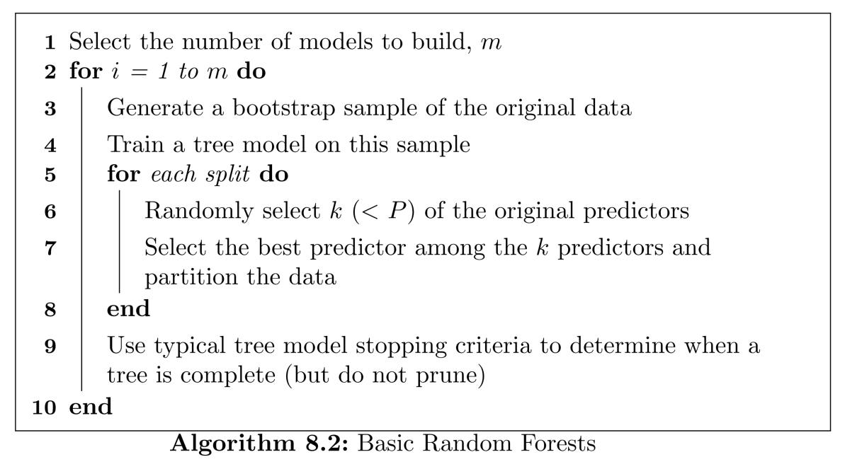
8.5 Random Forests
If we start with a sufficiently large number of original samples and a relationship between predictors and response that can be adequately modeled by a tree, then trees from different bootstrap samples may have similar structures to each other (especially at the top of the trees) due to the underlying relationship.
From a statistical perspective, reducing correlation among predictors can be done by adding randomness to the tree construction process.
After carefully evaluating these generalizations to the original bagging algorithm, Breiman constructed a unified algorithm called random forests.
Every model in the ensemble is then used to generate a prediction for a new ample and these m predictions are averaged to give the forest’s prediction.
Random forests’ tuning parameter is the number of randomly selected predictors, k, to choose from at each split. The practitioner must also specify the number of trees for the forest.
Compared to bagging, random forests is more computationally efficient on a tree-by-tree basis since the tree building process only needs to evaluate a fraction of the original predictors at each split, although more trees are usually required by random forests.
The ensemble nature of random forests makes it impossible to gain an understanding of the relationship between the predictors and the response.
Strobl et al. (2007) developed an alternative approach for calculating importance in random forest models that takes between-predictor correlations into account.

8.6 Boosting
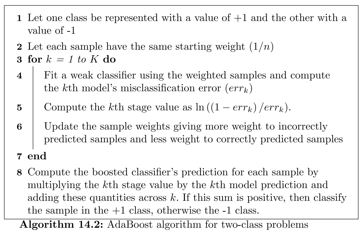
AdaBoost algorithm

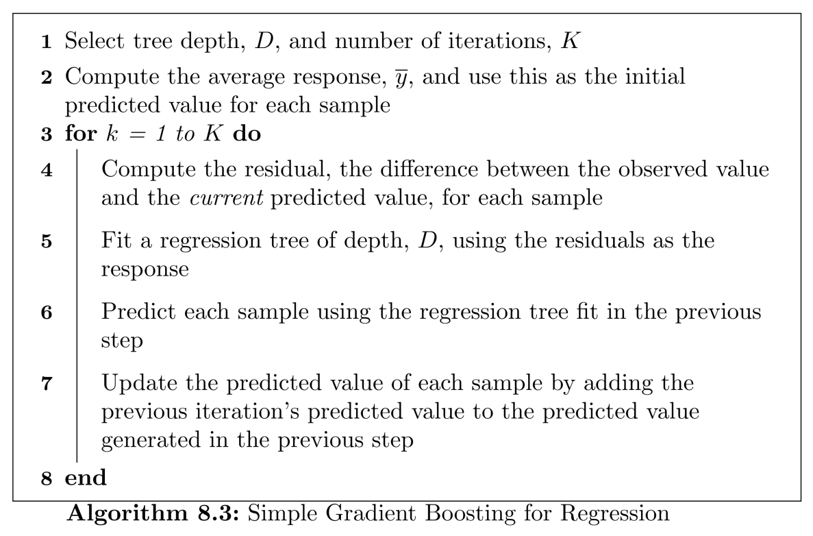
Gradient boosting machines
The basic principles of gradient boosting are as follows: given a loss function (e.g., squared error for regression) and a weak learner (e.g., regression trees), the algorithm seeks to find an additive model that minimizes the loss function.
When regression tree are used as the base learner, simple gradient boosting for regression has two tuning parameters: tree depth and number of iterations.
In random forests, all trees are created independently, each tree is created to have maximum depth, and each tree contributes equally to the final model. The trees in boosting, however, are dependent on past trees, have minimum depth, and contribute unequally to the final model.
A regularization strategy can be injected into the final line of the loop. Instead of adding the predicted value for a sample to previous iteration’s predicted value, only a fraction of the current predicted value is added to the previous iteration’s predicted value. This fraction is commonly
referred to as the learning rate and is parameterized by the symbol, λ. This parameter can take values between 0 and 1 and becomes another tuning parameter for the model.
Friedman updated the boosting machine algorithm with a random sampling scheme and termed the new procedure stochastic gradient boosting.

8.7 Cubist
Some specific differences between Cubist and the previously described approaches for model trees and their rule-based variants are:
• The specific techniques used for linear model smoothing, creating rules, and pruning are different
• An optional boosting—like procedure called committees
• The predictions generated by the model rules can be adjusted using nearby points from the training set data
y ̂_par=a×y ̂_k+(1-a)×y ̂_p
where y ̂_k is the prediction from the current model and y ̂_p is from parent model above it in the tree.
If the covariance is large, this implies that the residuals generally have the same sign and relative magnitude, while a value near 0 would indicate no (linear) relationship between the errors of the two models.
Let e_k be the collection of residuals of the child model and e_p be similar values for the parent model.
The smoothing coefficient used by Cubist is:
a=(Var[e_p ]-Cov[e_k,e_p])/(Var[e_p-e_k])
Var[e_p ] is proportional to the parent model’s RMSE.
The mth committee model uses an adjusted response
y_((m))^*=y-(y ̂_((m-1) )-y)
To tune this model, different numbers of committees and neighbors were assessed.

Tomorrow, I will start computing on Chapter 8.

Chapter 8 (8.3 8.4)

Today, I read Chapter 8 (8.3 8.4).

Summary

8.3 Rule-Based Models

The complexity of the model tree can be further reduced by either removing entire rules or removing some of the conditions that define the rule.

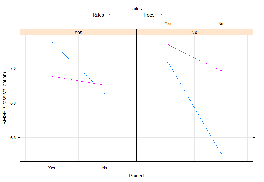
In figure 8.12, pruning has a large effect on the model and smoothing just has a large impact on the unpruned models.

The number of terms in the linear models decreases as more rules are created. This makes sense because there are fewer data points to construct deep trees.

8.4 Bagged Trees

Bagging, short for bootstrap aggregation, is a general approach that uses bootstrapping in conjunction with any regression model to construct an ensemble.

Advantages:

1.     Reduce the variance and be more stable (average)

2.     Provide their own internal estimate of predictive performance that correlates well with either cross-validation estimates or test set estimates (out-of-bag samples)

Most improvement in predictive performance is obtained aggregating across ten bootstrap replications.

Caveats:

1.     Computational costs and memory requirements increase as the number of bootstrap samples increases. (parallel computing)

2.     A bagged model is less interpretable than a model that is not bagged. (variable importance)

Next week, I will continue to read Chapter 8.