Summary
8.5 Random Forests
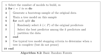
If we start with a sufficiently large number of original samples and a relationship between predictors and response that can be adequately modeled by a tree, then trees from different bootstrap samples may have similar structures to each other (especially at the top of the trees) due to the underlying relationship.
From a statistical perspective, reducing correlation among predictors can be done by adding randomness to the tree construction process.
After carefully evaluating these generalizations to the original bagging algorithm, Breiman constructed a unified algorithm called random forests.
Every model in the ensemble is then used to generate a prediction for a new ample and these m predictions are averaged to give the forest’s prediction.
Random forests’ tuning parameter is the number of randomly selected predictors, k, to choose from at each split. The practitioner must also specify the number of trees for the forest.
Compared to bagging, random forests is more computationally efficient on a tree-by-tree basis since the tree building process only needs to evaluate a fraction of the original predictors at each split, although more trees are usually required by random forests.
The ensemble nature of random forests makes it impossible to gain an understanding of the relationship between the predictors and the response.
Strobl et al. (2007) developed an alternative approach for calculating importance in random forest models that takes between-predictor correlations into account.
8.6 Boosting
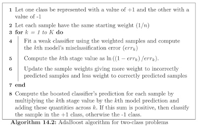
AdaBoost algorithm
Gradient boosting machines
The basic principles of gradient boosting are as follows: given a loss function (e.g., squared error for regression) and a weak learner (e.g., regression trees), the algorithm seeks to find an additive model that minimizes the loss function.
When regression tree are used as the base learner, simple gradient boosting for regression has two tuning parameters: tree depth and number of iterations.
In random forests, all trees are created independently, each tree is created to have maximum depth, and each tree contributes equally to the final model. The trees in boosting, however, are dependent on past trees, have minimum depth, and contribute unequally to the final model.
A regularization strategy can be injected into the final line of the loop. Instead of adding the predicted value for a sample to previous iteration’s predicted value, only a fraction of the current predicted value is added to the previous iteration’s predicted value. This fraction is commonly
referred to as the learning rate and is parameterized by the symbol, λ. This parameter can take values between 0 and 1 and becomes another tuning parameter for the model.
Friedman updated the boosting machine algorithm with a random sampling scheme and termed the new procedure stochastic gradient boosting.
8.7 Cubist
Some specific differences between Cubist and the previously described approaches for model trees and their rule-based variants are:
• The specific techniques used for linear model smoothing, creating rules, and pruning are different
• An optional boosting—like procedure called committees
• The predictions generated by the model rules can be adjusted using nearby points from the training set data
y ̂_par=a×y ̂_k+(1-a)×y ̂_p
where y ̂_k is the prediction from the current model and y ̂_p is from parent model above it in the tree.
If the covariance is large, this implies that the residuals generally have the same sign and relative magnitude, while a value near 0 would indicate no (linear) relationship between the errors of the two models.
Let e_k be the collection of residuals of the child model and e_p be similar values for the parent model.
The smoothing coefficient used by Cubist is:
a=(Var[e_p ]-Cov[e_k,e_p])/(Var[e_p-e_k])
Var[e_p ] is proportional to the parent model’s RMSE.
The mth committee model uses an adjusted response
y_((m))^*=y-(y ̂_((m-1) )-y)
To tune this model, different numbers of committees and neighbors were assessed.
Tomorrow, I will start computing on Chapter 8.


No comments:
Post a Comment